Excel Mortgage Amortization Schedule: Build One in 4 Steps
By Sohaib Ibrahim · Published November 11, 2026
To build an amortization schedule mortgage Excel users can reuse for any loan, type your loan amount, rate, and term into three cells, calculate the payment with the PMT function, and add one row per payment. Each row charges interest on the opening balance, sends the rest of the payment to principal, and carries the new balance to the next row. Add an extra payment column, then fill the formulas down 360 rows for a 30-year loan.
The problem is that a lender gives you a monthly payment and stops there. You do not see that on a $300,000 loan at 6.5%, only $271.20 of your first $1,896.20 payment reduces the balance. Free templates show the table, but many hide the formulas, assume monthly payments, or break the moment you add extra money.
This guide builds the sheet from scratch, so you control every formula. You get an input block, copy-ready formulas, extra-payment and biweekly options, and checks that prove the totals are right. We use the same $300,000 example throughout. HomeLoanCalc.io runs the same amortization math online, so you can use it to cross-check your sheet.
What you need before you build the sheet
An amortization schedule is a table that lists every loan payment, splits it into interest and principal, and shows the balance left afterward. You need Excel and four numbers: the loan amount, the annual rate, the term, and the number of payments per year.
What the schedule shows
Interest is charged on the remaining balance, so early payments are mostly interest. On the example loan, about 86% of the first payment ($1,625.00 of $1,896.20) is interest. Over 360 payments you pay roughly $382,600 in interest, more than the amount you borrowed.

The first years of a mortgage barely touch principal, which is why extra payments made early save the most.
This sheet models a fixed-rate loan and covers principal and interest only. Property tax, insurance, PMI, and HOA fees sit outside the table, so your lender's real bill will be higher if it escrows them.
Set up the input block
Label cells A1 to A6 and enter your values in column B. Keep every number you might change in this block, so no formula needs a hard-coded value later.
| Cell | Label | Example value |
|---|---|---|
| B1 | Loan amount | 300000 |
| B2 | Annual interest rate | 6.5% |
| B3 | Term in years | 30 |
| B4 | Payments per year | 12 |
| B5 | Scheduled payment | formula from Step 1 |
| B6 | Extra payment per period | 0 |
Step 1. Calculate the monthly payment
Enter =ROUND(-PMT(B2/B4, B3*B4, B1), 2) in cell B5 to get the scheduled payment. For the example loan it returns $1,896.20.
Enter the PMT formula
=ROUND(-PMT(B2/B4, B3*B4, B1), 2)
PMT needs three things: the rate per period (B2/B4), the number of payments (B3*B4), and the amount borrowed (B1). It returns a negative number because it treats the payment as money leaving your account, so the minus sign flips it. ROUND to two decimals matches how lenders bill.
PMT wants the rate per period and the number of periods, never the annual figures.
Avoid the three common input errors
Most wrong schedules trace back to one of these inputs:
- Rate typed as 6.5 instead of 6.5%. Excel reads 6.5 as 650%. Type the percent sign.
- Term entered in months. B3 is in years, and the formula multiplies by B4.
- A hard-coded 12 inside formulas. It works for monthly loans but breaks the weekly and biweekly versions in Step 3.
Step 2. Build the schedule rows
Put headers in row 8 and the first payment in row 9, then copy one row down 360 times. Every row uses the same logic: interest on the opening balance, principal as the rest of the payment, and a new ending balance.

Write the first row
Use these headers in A8:G8: Payment #, Beginning balance, Payment, Interest, Principal, Extra payment, Ending balance. Then enter the row 9 formulas below.
| Cell | Formula |
|---|---|
| A9 | 1 |
| B9 | =$B$1 |
| C9 | =MIN($B$5, B9+D9) |
| D9 | =ROUND(B9*$B$2/$B$4, 2) |
| E9 | =C9-D9 |
| F9 | =MIN($B$6, B9-E9) |
| G9 | =ROUND(B9-E9-F9, 2) |
Row 10 changes only two cells: A10 is =A9+1 and B10 is =G9. Copy C9:G9 down unchanged. The MIN functions stop the final payment and any extra payment from overshooting the balance, and the ROUND in column G makes the balance land on exactly 0.00.
Fill down and check the first rows
Select A10:G10 and drag the fill handle to row 368. That gives 360 rows for a 30-year monthly loan. For a longer term or more frequent payments, keep dragging until the balance hits zero. Rows after payoff simply show zeros.
Compare your first two rows with these figures:
| Payment # | Interest | Principal | Ending balance |
|---|---|---|---|
| 1 | 1,625.00 | 271.20 | 299,728.80 |
| 2 | 1,623.53 | 272.67 | 299,456.13 |
If you never plan extra payments, =-IPMT($B$2/$B$4, A9, $B$3*$B$4, $B$1) and the matching PPMT function return interest and principal for any payment number directly. The row-by-row method is better because it handles extra payments too.
If rows 9 and 10 match the table above, every row below them will be right.
Step 3. Add extra payments and compare
Type an amount in B6 and the schedule recalculates the payoff date and total interest. On the example loan, an extra $200 a month ends the loan at payment 277 instead of 360.
Enter a recurring extra amount
Set B6 to 200 and scroll to where the ending balance reaches zero. The comparison looks like this:
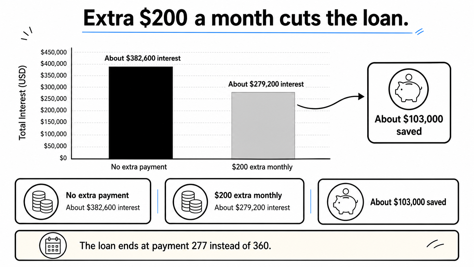
| Scenario | Payments | Payoff time | Total interest |
|---|---|---|---|
| No extra payment | 360 | 30 years | about $382,600 |
| $200 extra each month | 277 | 23 years 1 month | about $279,200 |
That saves roughly $103,000 in interest and shortens the loan by almost 7 years. Confirm with your lender that extra money is applied to principal and that no prepayment penalty applies.
Because extra money goes straight to principal, every later row charges less interest than it did before.
Add a one-time lump sum
Add two inputs in D1:E2: a payment number in E1 (for example 24) and an amount in E2 (for example 10000). Then replace the formula in F9 and copy it down:
=MIN($B$6+IF(A9=$E$1,$E$2,0), B9-E9)
A bonus or tax refund now hits exactly the payment you chose, and every row after it recalculates.
Model weekly and biweekly payments
For a true biweekly loan, set B4 to 26 and fill down 780 rows. For weekly, set B4 to 52 and fill down 1,560 rows. The PMT and interest formulas adjust on their own because they divide by B4.
Many lenders instead offer a plan that pays half the monthly payment every two weeks, which equals 13 monthly payments a year. Keep B4 at 12 and set B6 to =B5/12, about $158.02 here, to approximate it.
Step 4. Check your totals and save the file
Four summary formulas prove the schedule is right, and a few print settings turn it into a PDF you can share. Run the checks before you rely on any number.
Verify the schedule
Put these checks below or beside the table:
| Check | Formula | Should equal |
|---|---|---|
| Total interest | =SUM(D9:D368) |
about $382,600 with no extra payment |
| Principal repaid | =SUM(E9:F368) |
the loan amount in B1 |
| Final balance | =G368 |
0 |
| Total paid | =SUM(C9:C368)+SUM(F9:F368) |
loan amount plus total interest |
Then compare D9 with the interest line on your first lender statement. A difference of a few cents can come from rounding or day-count rules, but a gap of dollars means an input is wrong. Treat the result as a planning estimate, because your lender's actual figures can differ slightly.
If principal repaid does not equal the loan amount, a formula was not copied down all the way.
Print it, save it, or cross-check it online
To print, use Page Layout, then Print Titles, and set row 8 as the row to repeat at the top. In the print dialog, choose Save as PDF for a printable amortization schedule. Excel's own templates under File, then New, offer a quick start, but you should still trace each template's numbers back to formulas like these.
For a second opinion, the HomeLoanCalc.io Amortization Calculator builds a schedule from loan amount, rate, and term, with a toggle between annual and monthly views. The Extra Mortgage Payment Calculator compares your original payoff with an accelerated one, and the Mortgage Calculator adds taxes, insurance, PMI, and HOA fees. All three are free with no signup.
Your schedule is ready to use
You now have a working mortgage schedule: one PMT formula for the payment, seven columns that split each payment into interest and principal, and an extra payment column that shows what each additional dollar saves. The check formulas tell you when the sheet is right.
Save the file, change the inputs when rates or plans change, and rerun the checks. To compare scenarios without rebuilding anything, try the free HomeLoanCalc.io calculators and see your payoff schedule in seconds.
This article is for general information and is not financial advice. Confirm figures with your lender or an official source before you decide.
Run your own numbers
Use our free calculators to see what this means for your loan.
More articles
- $60K Salary Home Budget: How Much House Can You Afford?
- How Much House Can I Afford with 300K Salary? Step by Step
- Longest Mortgage Term: Do 40- and 50-Year Loans Exist?
- How Much House Can I Afford with 70K Salary? $170K to $305K
- FHA Debt-to-Income Ratio Calculator: How to Check 31/43
- Mortgage Insurance Disbursement: What the Line Item Means
- Current FHA Interest Rates: What Sets Your 30-Year Rate
- Mortgage Calculator with Tax and Insurance: How to Use It
- How Much Down Payment Do You Need for a 500K House?
- How Much to Afford a 500K House: Income and Down Payment